Exponentially weighted moving average

This algorithm is one of the most important algorithms currently in usage. From financial time series, signal processing to neural networks , it is being used quite extensively. Basically any data that is in a sequence.

We mostly use this algorithm to reduce the noise in noisy time-series data. The term we use for this is called “smoothing” the data.

The way we achieve this is by essentially weighing the number of observations and using their average. This is called as Moving Average.

This method is effective however, it is not very easy to do as it involves holding the past values in memory buffer and constantly updating the buffer whenever a new observation is read. Here is where EWMA comes into picture.

EWMA solves this problem with a recursive formula.

fig. EWMA formula

Formula Explanation :

The formula states that the value of the moving average(S) at time t is a mix between the value of raw signal(x) at time t and the previous value of the moving average itself i.e. t-1. The degree of mixing is controlled by the parameter a (value between 0–1).

So, if a = 10%(small), most of the contribution will come from the previous value of the signal. In this case, “smoothing” will be very strong.

if a = 90%(large), most of the contribution will come from the current value of the signal. In this case, “smoothing” will be minimum.

So for a better understanding, we will consider an example of “temperature variation on the weekdays of a week” data.

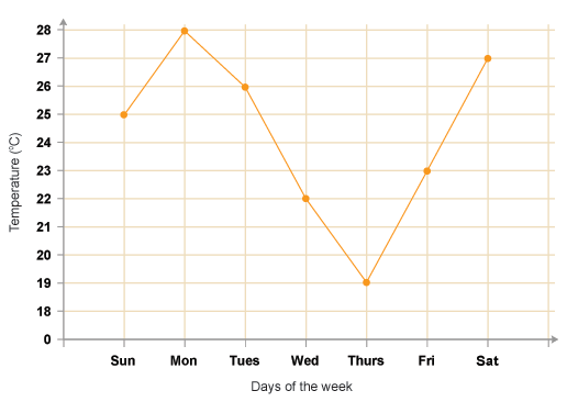
fig. Temp vs days of the week

Now as you can see, we need to “smoothen” out the above graph to have consistency in data.

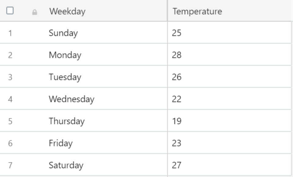
fig. The data for temp. vs weekdays

Now let us take a = 10%, considering the new formula will be:

fig. EWMA formula for a=10%

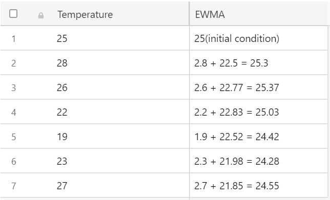
fig. calculation of EWMA

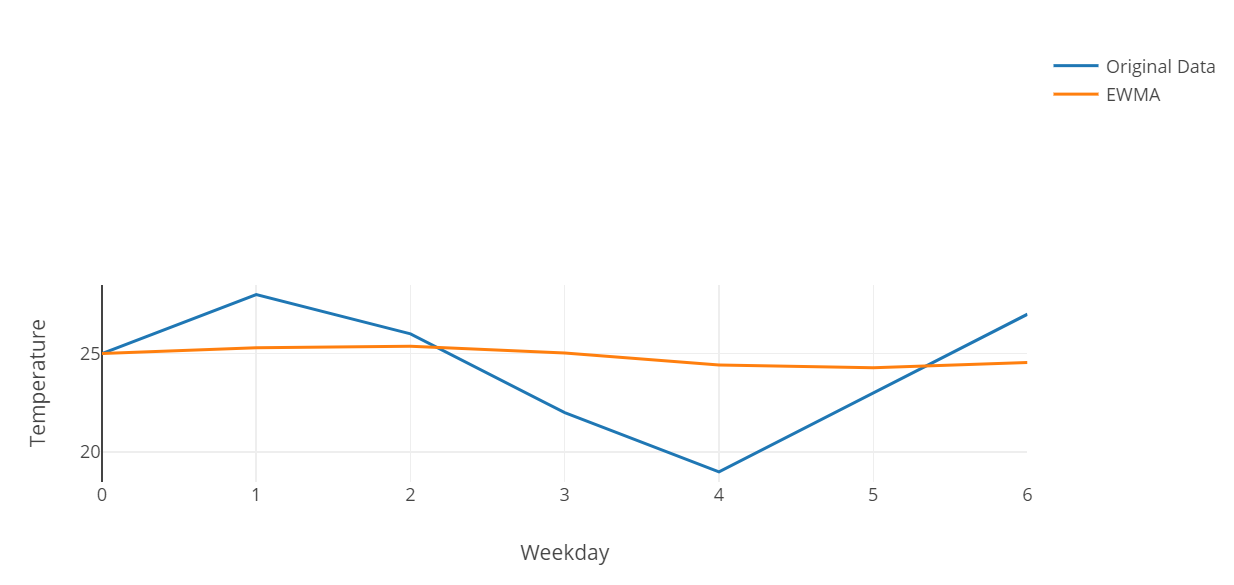
fig. Original graph vs EWMA

As we can see, a =10% provides really strong smoothing.

To summarize, we have introduced EWMA and have solved a sample dataset to see how time series/sequential data is smoothed out for use in various algorithms.